
Polarith AI


1.8
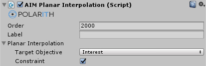
front-end / back-end: AIMPlanarInterpolation | PlanarInterpolation
inherits from: AIMBehaviour | MoveBehaviour
Planar Interpolation solves the major problem of using a discrete sensor. The number of possible solutions and, thus, possible movement directions are limited by the available receptors, but agents live in a continuous world. So it is highly recommended to use this behaviour for your agents to keep the sensor's receptor count low (to save performance) and the movement of your agents smooth.
This component has got the following specific properties.
| Property | Description |
|---|---|
TargetObjective | Specifies the objective which should be the basis for the calculations. It is recommended to use the objective which represents interest. |
Constraint | If the interpolator finds a better solution, it is possible that this solution violates one of the set constraints. If this setting is enabled, the solution is rejected if at least one constraint is exceeded. |
The Order of this behaviour is set to 2000 which is also the allowed minimum for this component. Because of this, the processing of this behaviour is forced to take place after the MCO solver have found a solution. This is important since an already made decision is the basis for the interpolation to work properly.
The following Figure 1 demonstrates the effect an active Planar Interpolation has on the movement if using a sensor with a relatively low receptor count (~16).
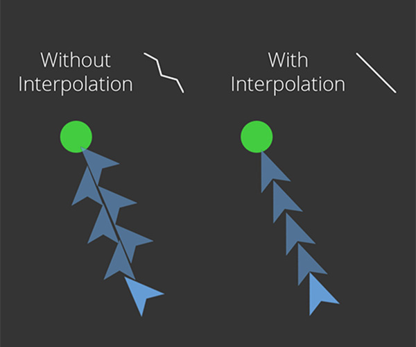
Figure 1: At the left, the resulting trajectory of an agent with low sensor resolution can be seen. Instead of moving straight to the target, this agent oscillates around the direct continuous path. At the right, there is a similar agent with interpolation enabled. It follows the direct path as to be expected.
Without interpolation, the internal MCO solver would oscillate between 2 solutions represented by two distinct receptors. Figure 1 shows the result, whereby the agent at the left is not able to move on a straight path to the target due to the discrete nature of the applied sensor. So there is only a finite number of directions that the agent can base its movement decisions on.
To overcome this disadvantage, linear interpolation can be applied. The intention is to find a better solution nearby the original solution provided by the solver. First, a TargetObjective must be defined, whereby we advise to use the interest objective for this purpose. Based on adjacent objective values, two lines are defined (as can be seen in Figure 2). By solving the resulting linear equations, a possible better solution can be found. The solution is used as the new result only if the following two conditions hold true.
Constraint flag is enabled, the resulting objective values must not exceed the given constraints for all other objectives.If such a solution is found, the interpolation parameter t is calculated based on the TargetObjective's solution. With this parameter the other objective values are calculated by linear interpolation.
Other alternatives would be, on the one hand, to increase the ReceptorCount (which decreases performance a lot) or, on the other hand, to use a physics controller which naturally tends to smooth the movement of an agent. However, we advise to prefer the use of the Planar Interpolation behaviour because it is the best compromise between use and performance. By the way, a physics controller does not solve the problem at all, it just hides it.
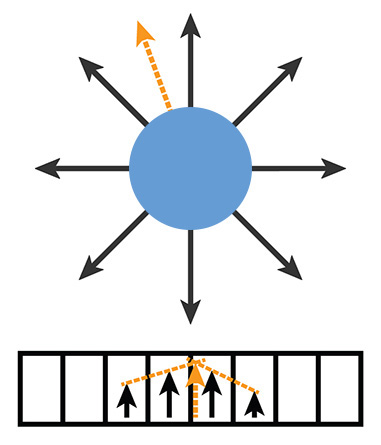
Figure 2: Depicts the interpolation mechanism. For the TargetObjective, a potential better solution is calculated by solving a system of linear equations. The lines are based on adjacent objective values like it is shown at the bottom of this image.